

If you have three or more groups to compare and SPSS is sitting open in front of you, take a breath. Learning how to run a one-way ANOVA in SPSS is one of the most common tasks in a dissertation results chapter — and it is very learnable.
In this case study we run a complete one-way ANOVA in SPSS together, slowly: setting up the data, every click, every output table explained, and a finished APA-style results paragraph at the end. No panic, no unexplained jargon — one small step at a time.
In this guide
- What is a one-way ANOVA — and when do you use it?
- The case study: does study support change exam performance?
- The hypotheses
- Setting up your data (2 minutes that save hours)
- Running the ANOVA: Steps 1-5
- Reading the output: Steps 6-9
- Step 10 — Effect size
- The APA-style write-up
- Common mistakes (and calm fixes)
- Quick questions, answered
What Is a One-Way ANOVA (and When Do You Use It)?
A one-way ANOVA compares the means of three or more groups on one continuous outcome. Use it when:
- You have one grouping variable with three or more groups (three teaching methods, four age bands).
- You have one continuous outcome for everyone (a test score, a scale total, time taken).
- Each person belongs to only one group.
Why not just run several t-tests? A t-test compares only two groups. Run three t-tests instead of one ANOVA and each test brings its own chance of a misleading significant result — and those chances add up.
ANOVA tests all your groups in one go. Then a follow-up test, called a post-hoc test, points to exactly which groups differ. That is the whole logic — everything below follows from it.
The Case Study: Does Study Support Change Exam Performance?
Our worked example is a realistic dissertation scenario — the kind of study students bring to us every week.
A student researcher asked whether the type of study support students used during the term made a difference to their academic performance. Ninety undergraduate students took part, each in exactly one group:
- Group 1 — No extra support: students studied on their own, as usual.
- Group 2 — Peer study group: weekly small groups, led by students.
- Group 3 — Tutor-led sessions: weekly support sessions led by a tutor.
At the end of term, all 90 students sat the same standardised test, scored out of 100.
Research question: Does the type of study support make a difference to students’ academic performance scores?
Why ANOVA fits: one continuous outcome (test score), one grouping variable with three groups. A t-test cannot compare three groups at once — that single sentence is why this analysis begins with a one-way ANOVA.
Practise along with us: download the exact practice dataset used here — download the free ANOVA practice dataset (CSV) — and follow every step in your own SPSS. If your numbers match ours at the end, you have done it perfectly. (It is a teaching dataset created for this case study, so you can learn the method safely before touching your own data.)
The Hypotheses
Every ANOVA starts with two statements:
- H0 (null hypothesis): There is no difference in mean academic performance scores between the three study support groups.
- H1 (alternative hypothesis): There is a difference in mean academic performance scores between at least two of the three groups.
Notice the careful wording of H1: at least two groups. ANOVA tells you that a difference exists somewhere — not which groups differ. Finding that out is the post-hoc test’s job (Step 9). Examiners look for this distinction, so it is worth understanding from the start.
Before You Run Anything: Setting Up the Data
Five calm minutes here will save you confusion everywhere else. Your SPSS file needs just two variables:
| Variable | Type | Measure | What to set |
|---|---|---|---|
| Group | Numeric | Nominal | Value labels: 1 = No extra support, 2 = Peer study group, 3 = Tutor-led sessions |
| Score | Numeric | Scale | The test score out of 100. Decimals: 0 is fine for whole-number scores |
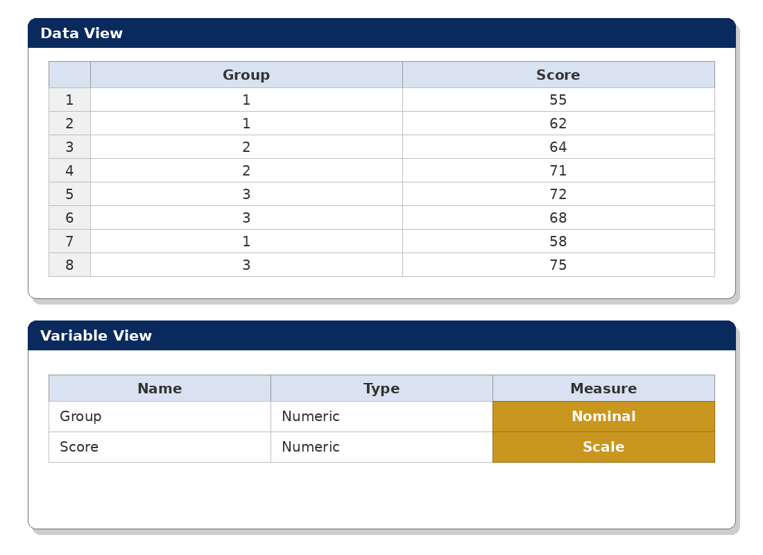
In Data View, each row is one student: their group code (1, 2 or 3) and their score. Before testing, run two quick sanity checks:
- Analyze → Descriptive Statistics → Frequencies on Group — you should see 30 students per group, 90 in total.
- Descriptives on Score — to spot anything impossible, like a score of 999 from a missed decimal point.
Catching a typo now is far calmer than explaining a strange result later.
Step by Step: Running the One-Way ANOVA in SPSS
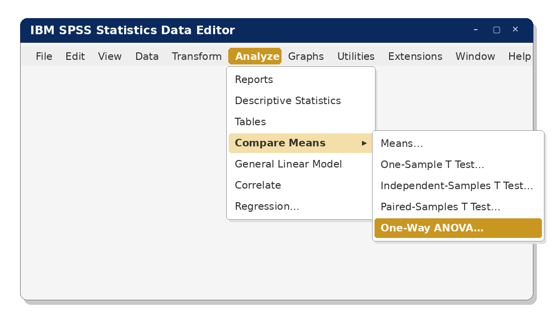
Step 1 — Open the test
Click Analyze → Compare Means → One-Way ANOVA… A dialogue box opens. Nothing has happened to your data — you can close this box at any point and nothing changes.
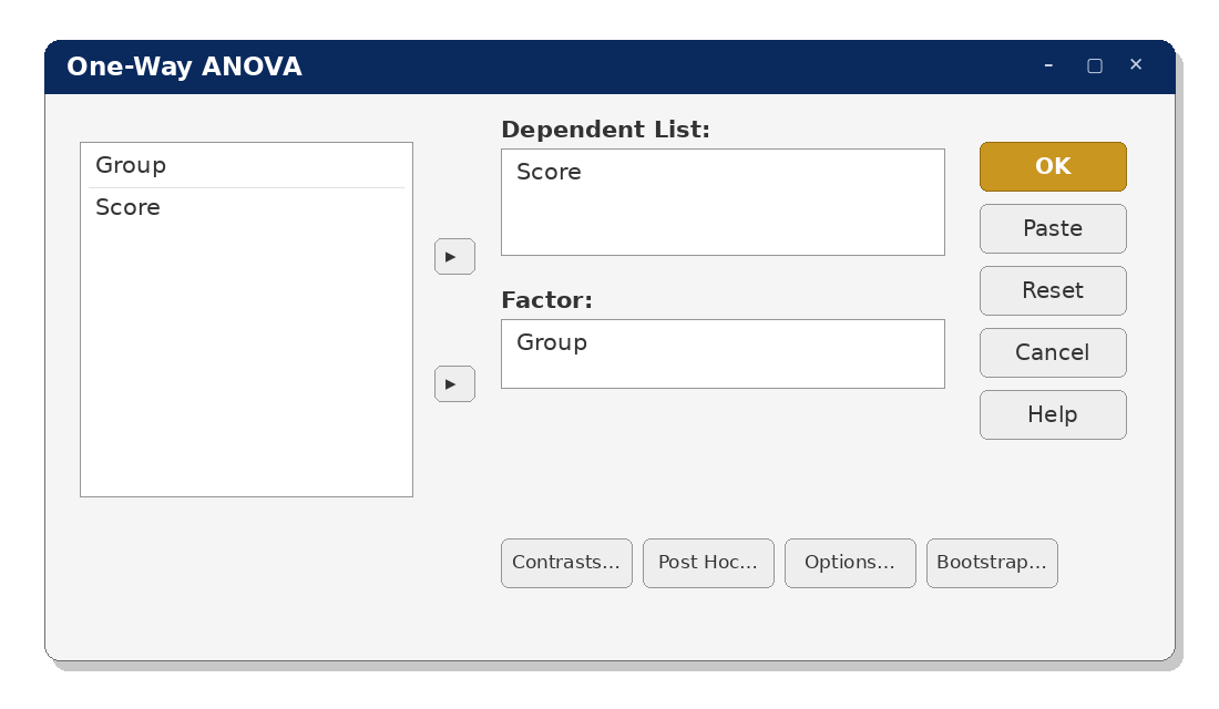
Step 2 — Assign your variables
Move Score into the Dependent List box (the outcome), and Group into the Factor box (the grouping variable). Easy way to remember: the factor is what sorts students into groups; the dependent variable is what you measured.
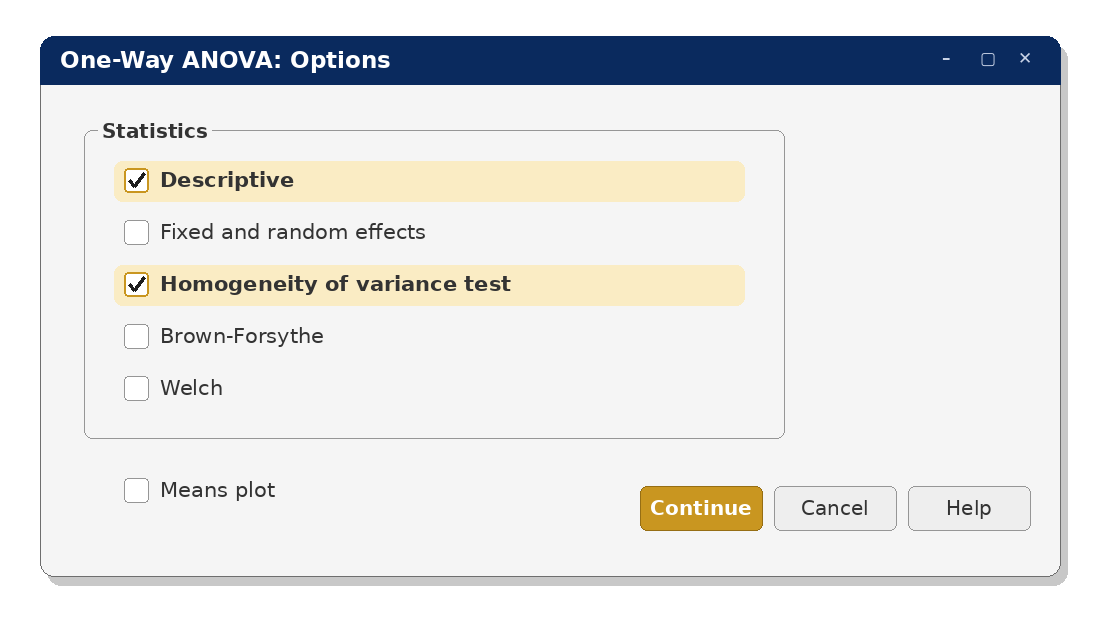
Step 3 — Ask for descriptives and the variance check
Click Options…, tick Descriptive and Homogeneity of variance test, then Continue. These two ticks give you the group means table and Levene’s test, which checks an ANOVA assumption for you.
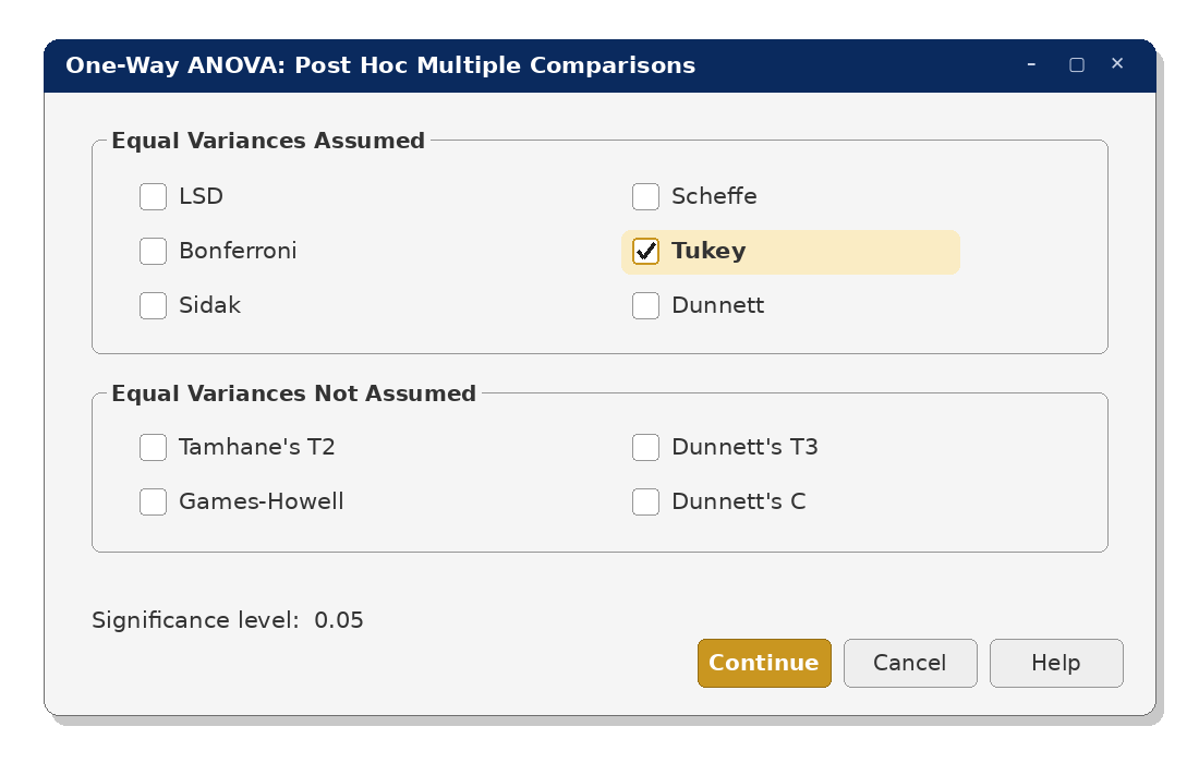
Step 4 — Choose the post-hoc test
Click Post Hoc… and tick Tukey, then Continue. Tukey is the standard choice when group variances are roughly equal — which Step 3’s Levene test is about to confirm. (If variances turn out very unequal, the calm alternative is the Welch ANOVA with Games-Howell post-hoc — covered fully in our assumptions case study.)
Step 5 — Run it
Click OK. The Output window opens with four tables. And if SPSS makes you nervous, remember: running an analysis never changes or damages your data. You can re-run it as many times as you need. Now let’s read each table, in the order SPSS gives them.
Reading the Output, Table by Table
Step 6 — The Descriptives Table: Look at the Means First
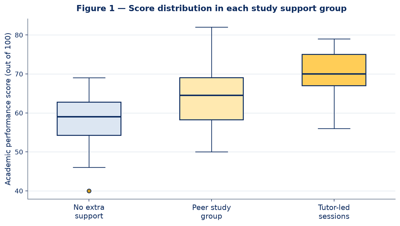
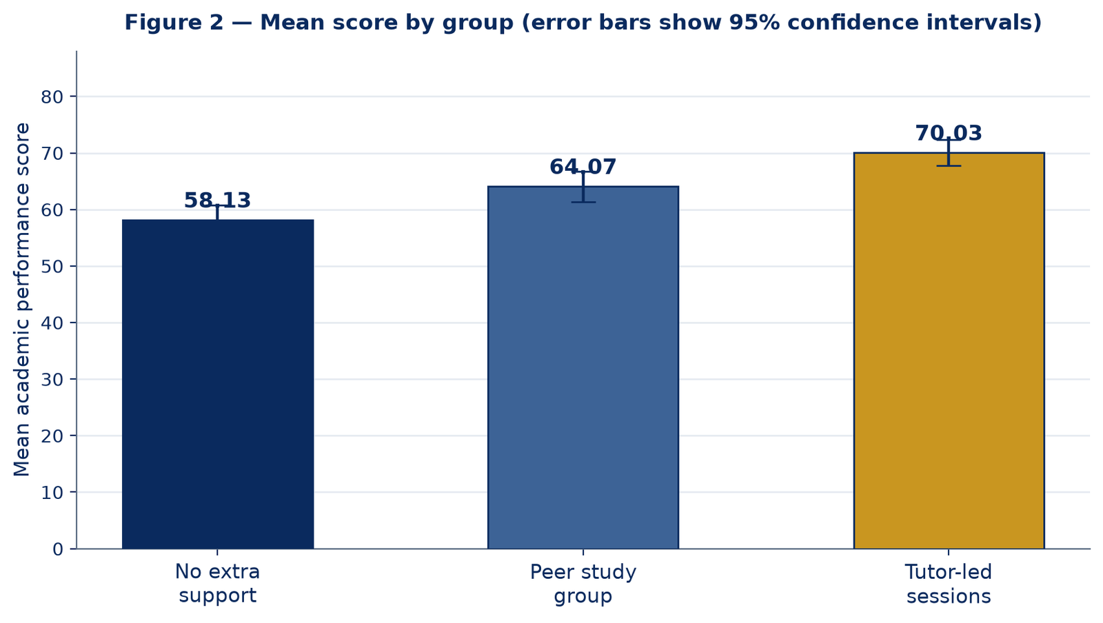
Before any p-value, look at the pattern with your own eyes. Do the groups look different?
Table 1. Descriptives — Academic performance score
| Group | N | Mean | SD | SE | 95% CI | Min | Max |
|---|---|---|---|---|---|---|---|
| No extra support | 30 | 58.13 | 7.06 | 1.29 | 55.50 – 60.77 | 40 | 69 |
| Peer study group | 30 | 64.07 | 7.24 | 1.32 | 61.36 – 66.77 | 50 | 82 |
| Tutor-led sessions | 30 | 70.03 | 6.06 | 1.11 | 67.77 – 72.30 | 56 | 79 |
| Total | 90 | 64.08 | 8.32 | 0.88 | 62.34 – 65.82 | 40 | 82 |
What this means: the tutor-led group scored highest on average (M = 70.03), then the peer group (M = 64.07), then no support (M = 58.13). The SDs (around 6–7 in every group) show scores were similarly spread out in all three groups. The pattern already matches the research expectation — but seems is not enough for a dissertation. The next tables test whether these gaps are bigger than ordinary random variation.
Step 7 — Levene’s Test: Checking the Variances Assumption
A one-way ANOVA assumes the groups have roughly equal variances — scores spread out about as much in each group. Levene’s test checks this for you.
Table 2. Test of Homogeneity of Variances
| Levene Statistic | df1 | df2 | Sig. (p) |
|---|---|---|---|
| 0.384 | 2 | 87 | .682 |
What this means: here, a non-significant result is what you want. Because p = .682 (greater than .05), the variances are similar enough — the assumption is met, and you can trust the standard ANOVA and Tukey test that follow. One less thing to worry about. (If Levene’s test is ever significant in your own work: don’t panic — use the Welch ANOVA and Games-Howell post-hoc, and say so in one sentence.)
Step 8 — The ANOVA Table: The Overall Answer
This is the headline table. It answers one question: is there a statistically significant difference somewhere between the group means?
Table 3. One-Way ANOVA — Academic performance score
| Source | Sum of Squares | df | Mean Square | F | Sig. (p) |
|---|---|---|---|---|---|
| Between Groups | 2124.16 | 2 | 1062.08 | 22.93 | < .001 |
| Within Groups | 4030.30 | 87 | 46.33 | ||
| Total | 6154.46 | 89 |
How to read it, column by column:
- Between Groups — variation explained by group membership. This is what your research question is about.
- Within Groups — ordinary variation between individual students inside each group. The background noise.
- F = 22.93 — essentially the signal compared with the noise. Much larger between than within produces a large F.
- Sig. (p) < .001 — the decision-maker. (SPSS prints .000 — you never write p = .000; the correct report is p < .001.)
The decision: because p < .05, we reject H0. There is a statistically significant difference in scores somewhere between the three groups: F(2, 87) = 22.93, p < .001. But remember H1‘s careful wording — this table alone does not say which groups differ. For that, we need the final table.
Step 9 — The Tukey Post-Hoc Test: Which Groups Actually Differ?
The Multiple Comparisons table compares every pair of groups. Read each row’s Mean Difference, Sig. and confidence interval together. An asterisk (*) means that pair differs significantly at the .05 level.
Table 4. Multiple Comparisons (Tukey HSD)
| Group (I) | Group (J) | Mean Difference (I − J) | SE | Sig. (p) | 95% CI |
|---|---|---|---|---|---|
| No extra support | Peer study group | −5.93* | 1.76 | .003 | −10.12 to −1.74 |
| No extra support | Tutor-led sessions | −11.90* | 1.76 | < .001 | −16.09 to −7.71 |
| Peer study group | Tutor-led sessions | −5.97* | 1.76 | .003 | −10.16 to −1.78 |
* The mean difference is significant at the .05 level. (SPSS shows each pair twice, in both directions; the three unique comparisons are shown here.)
What this means, pair by pair:
- Peer vs No support: peer group scored 5.93 marks higher (p = .003).
- Tutor-led vs No support: tutor-led scored 11.90 marks higher — the largest gap (p < .001).
- Tutor-led vs Peer: tutor-led scored 5.97 marks higher (p = .003).
All three groups differ from each other. Any support beat studying alone, and tutor-led support beat peer support. Never stop at the ANOVA was significant — this detail is what your results chapter needs.
Reading along nicely? If choosing the right test is the part you feel unsure about, our free workbook — SPSS Dissertation Workbook: Which Test Should You Use? — walks you through the choice in a few gentle questions. Get the free workbook. And if your own data is where you’re stuck, tap the WhatsApp icon and tell us where — a second pair of eyes, calmly, no pressure.
Step 10 — Effect Size: How Big Is the Difference?
A p-value tells you a difference is unlikely to be a fluke. An effect size tells you whether it is big enough to matter.
For a one-way ANOVA the common measure is eta squared (η²) — the proportion of all variation in scores that group membership explains. You can calculate it straight from Table 3:
η² = Sum of Squares (Between Groups) ÷ Sum of Squares (Total) = 2124.16 ÷ 6154.46 = .35
So about 35% of the variation in test scores is explained by which support group a student was in. Using the usual benchmarks (.01 = small, .06 = medium, .14 = large), η² = .35 is a large effect.
(In newer SPSS versions you can also tick Estimates of effect size in the Options box and SPSS prints eta squared for you.) Not every supervisor asks for an effect size — but reporting one is a quiet mark of a careful researcher.
Writing It Up: The APA-Style Results Paragraph
Here is the complete analysis as a finished results paragraph, in APA style, using the real values from the tables above. Notice how every number earns its place — and how the paragraph still makes sense to a reader who never sees the tables.
A one-way ANOVA was conducted to compare academic performance scores across the three study support groups. Levene’s test indicated that the assumption of homogeneity of variances was met, F(2, 87) = 0.38, p = .682. There was a statistically significant difference in scores between the groups, F(2, 87) = 22.93, p < .001, η² = .35. Post-hoc comparisons using the Tukey HSD test indicated that the mean score for the tutor-led group (M = 70.03, SD = 6.06) was significantly higher than for the peer study group (M = 64.07, SD = 7.24), p = .003, and the no-support group (M = 58.13, SD = 7.06), p < .001. The peer study group also scored significantly higher than the no-support group, p = .003. These findings suggest that tutor-led study support was associated with the highest academic performance in this sample.
Two style details worth copying: F, df and p are always reported together. And because this study compared groups rather than randomly assigning students in a controlled experiment, the paragraph says the support was associated with higher performance — it does not claim ANOVA proved the support caused it. Examiners notice that care.
So, What Does This Case Study Show?
In this case study, the type of study support did make a difference. Tutor-led students scored highest, peer-group students next, and students without extra support lowest — and the post-hoc test showed us exactly which groups differed.
That is the whole job of a one-way ANOVA: one clear overall answer first, then the detail of where the difference is. If your dissertation compares three or more groups on one outcome, this is a test you can now run and write up with confidence.
New to SPSS entirely? Start with our SPSS help and case studies hub — every guide follows this same calm, step-by-step format.
Common Mistakes (and the Calm Fix for Each)
- Running three t-tests instead of one ANOVA. Multiple t-tests inflate the chance of a false significant finding. One ANOVA plus a post-hoc test is the correct, cleaner route.
- Forgetting value labels, or leaving Group set to Scale. Two minutes in Variable View — Group as Nominal with labels, Score as Scale — saves confusion everywhere later.
- Reporting only p = .000. SPSS prints .000 when p is smaller than .001. Write p < .001, and always report F, df, the group means and SDs alongside.
- Stopping at the ANOVA table. A significant ANOVA only says a difference exists somewhere. The post-hoc table says where — and examiners look for it.
- Claiming ANOVA proves one group caused the difference. Unless your design was a true experiment with random assignment, write about differences and associations, not proof of cause.
- Panicking when Levene’s test is significant. A known, solvable situation: use the Welch ANOVA and Games-Howell post-hoc, and say so in one sentence.
Frequently Asked Questions
Count your groups. Two groups → an independent-samples t-test. Three or more groups on one continuous outcome → a one-way ANOVA. If you are unsure which test your research question needs at all, our free workbook below walks you through the choice in a few gentle questions.
Your variances are quite different between groups. Stay calm: in the One-Way ANOVA dialogue, tick Welch in Options, and choose Games-Howell as your post-hoc test instead of Tukey. Then report the Welch F and say in one sentence why you used it.
After a significant ANOVA, the post-hoc test compares every pair of groups while keeping the overall error rate under control. It turns something differs into the tutor-led group scored higher than both other groups — the detail your discussion chapter needs.
If your university or supervisor follows APA style closely, yes — eta squared (η²) is the standard choice, and you can calculate it from the ANOVA table as shown in Step 10, or ask SPSS to print it via Options → Estimates of effect size.
Probably not. A non-significant result (p >.05) simply means the group differences in your data could plausibly be ordinary variation — a legitimate finding, reported honestly in exactly the same format, minus the post-hoc test (which you do not run when the overall test is not significant).
Keep learning — students also read
- SPSS Help & Case Studies Hub — every guide, one calm place
- Free Workbook: Which Test Should You Use? — choose your test in minutes
- Coming next: Setting Up Your Data in SPSS · Which Test Should You Use? · Two-Way ANOVA in SPSS
You have just worked through a complete ANOVA — well done.
If choosing the right test is the part you still feel unsure about, take our free workbook: SPSS Dissertation Workbook — Which Test Should You Use? It walks you through the choice in a few simple questions.
Prefer something printable? Our Etsy shop has thesis planners and SPSS checklists made for dissertation students.
Also from us: Confident Viva — calm, practical viva preparation for PhD and Masters students.
And if you are working with your own data and would like a second pair of eyes, message us on WhatsApp — tap the icon, tell us where you got stuck, and we will help you find your next step, calmly. No pressure, ever.
Stuck on a step, or did your output look different? Ask in the comments below — we read and reply to every student’s question.
Next in this series: How to Run a Two-Way ANOVA in SPSS — Step-by-Step Case Study
Pingback: Two-Way ANOVA in SPSS: Step-by-Step Case Study | Results Chapter