
Our paired t-test case study compared the same students at two timepoints, and the independent t-test before it compared two groups. But many dissertations ask a different kind of question — not “do groups differ?” but “do two things move together?” When both of your variables are numbers, you need correlation: the calmest way to measure a relationship in SPSS.
In this case study we run a complete Pearson correlation together: the setup, every click, every output table explained, the scatterplot check, and a finished APA-style results paragraph. One small step at a time.
In this guide
- What Pearson’s correlation is — and when to use it (vs Spearman)
- The case study: do students who revise more score higher?
- The hypotheses (one pair, one relationship)
- Setting up your data
- Running the correlation: Steps 1–3
- Reading the output: Steps 4–6
- The APA-style write-up
- Common mistakes (and calm fixes)
- Quick questions, answered
What Is Pearson’s Correlation (and When Do You Use It)?
Pearson’s r measures how strongly two continuous variables move together in a straight line — from −1 (perfect negative) through 0 (no line at all) to +1 (perfect positive). Use it when:
- You have two continuous variables — hours and marks, anxiety and sleep, age and income.
- Each person (or case) has one score on each — 80 students, two numbers each.
- The relationship looks roughly straight-line on a scatterplot (we will check this).
When would you use Spearman instead? When at least one variable is ordinal (rankings, Likert-scale items you are treating as ranks), or when the relationship is monotonic but curved, or when outliers are dragging Pearson around. Same SPSS dialogue box — you just tick a different box. This case study is Pearson; the Spearman tick-box is one click away when you need it.
The Case Study: Do Students Who Revise More Score Higher?
Danish is writing his master’s dissertation on study habits. He surveyed 80 coursemates, asking each of them two simple questions: how many hours a week do you revise? and what was your final exam mark? His supervisor looked at the spreadsheet and asked, “So — is there actually a relationship here?” Danish froze. He had only ever compared groups. Nobody had taught him how to relate two numbers.
Research question: is there a relationship between weekly revision hours and exam scores?
Why Pearson fits: two continuous variables, one score per student on each, and (as the scatterplot will confirm) a roughly straight-line pattern. A t-test here would be nonsense — there are no groups to compare, only pairs of numbers.
Practise along with us: download the practice dataset used here — download the free correlation practice dataset (CSV) — and follow every step in your own SPSS.
The Hypotheses
One pair of hypotheses, stated as a relationship:
- H0 — there is no linear relationship between revision hours and exam scores in the population (r = 0).
- H1 — there is a linear relationship between revision hours and exam scores (r ≠ 0).
Before You Run Anything: Setting Up the Data
Correlation needs the simplest layout of all: one row per person, one column per variable.
| Variable | Type | Measure | What to set |
|---|---|---|---|
| StudentID | Numeric | Nominal | One row per student (1–80) |
| StudyHours | Numeric | Scale | Revision hours per week |
| ExamScore | Numeric | Scale | Final exam mark (0–100) |
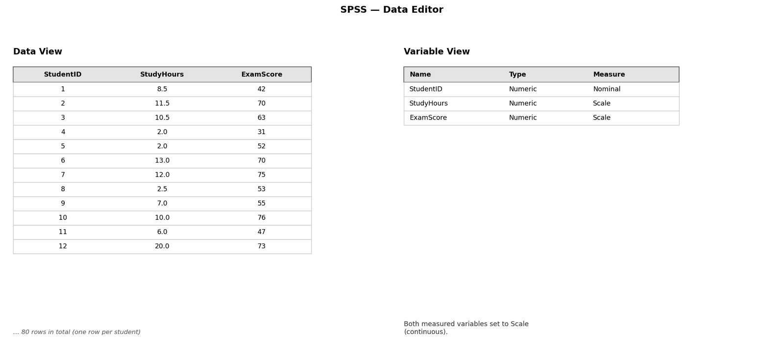
Both measured variables must be set to Scale in Variable View — that is SPSS’s word for continuous. Quick sanity check before anything else: Descriptives on both variables to catch impossible values (an exam score of 900, a revision week of 200 hours).
Step by Step: Running the Correlation in SPSS
Step 1 — Open the test
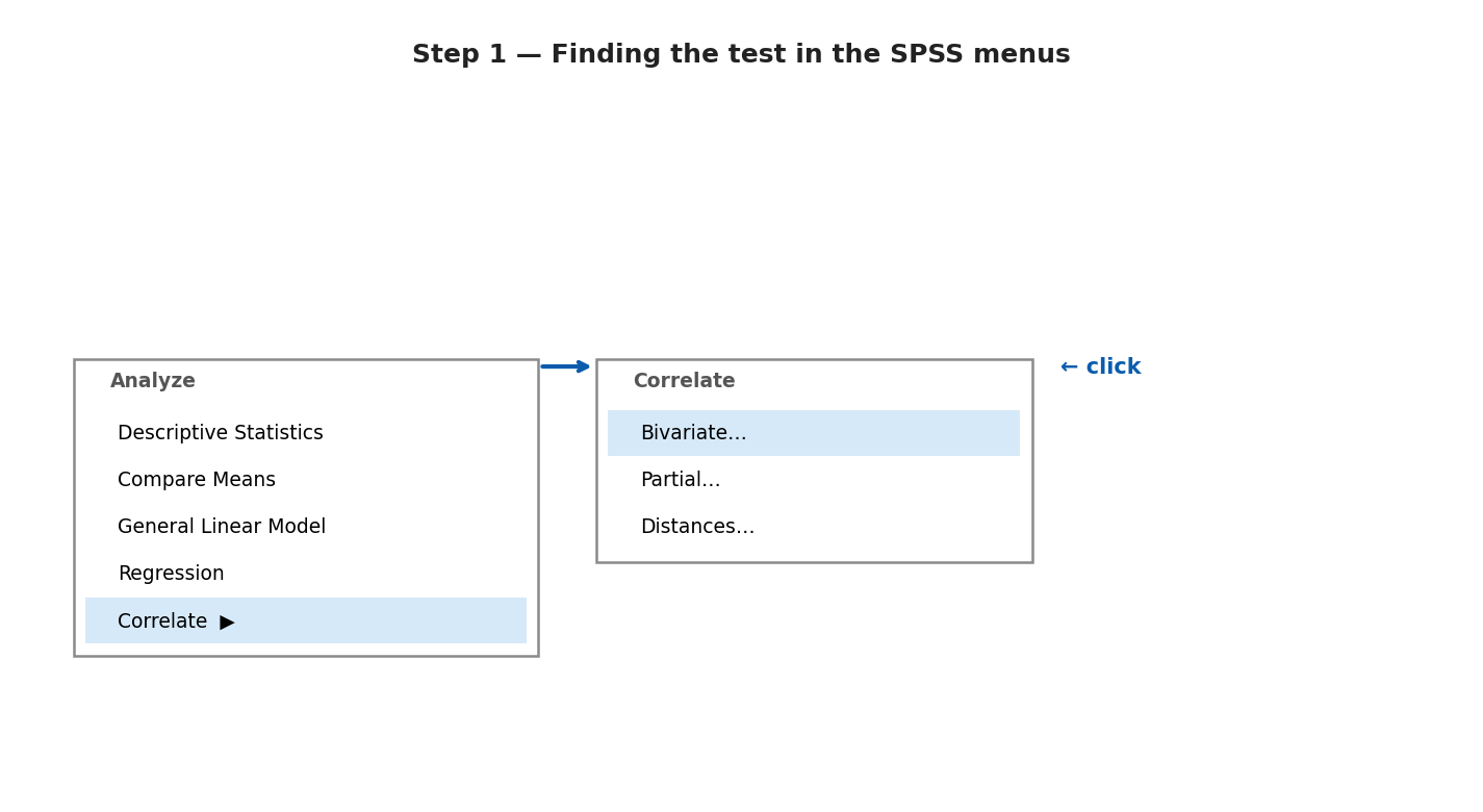
Click Analyze → Correlate → Bivariate… A dialogue box opens.
Step 2 — Move your variables and tick the right boxes
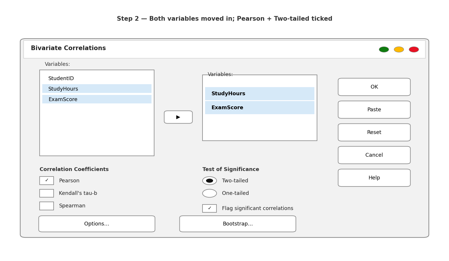
Move StudyHours and ExamScore into the Variables box. Under Correlation Coefficients, Pearson is already ticked — that is the one we want. Under Test of Significance, leave Two-tailed ticked (our hypothesis did not predict a direction). Keep Flag significant correlations ticked — it puts helpful stars next to significant results.
Step 3 — Run it
Click OK. The Output window opens with one small table. The whole analysis fits on a postcard — correlation is the gentlest test in this series.
Reading the Output, Table by Table
Step 4 — Descriptives First: Meet Your Two Variables
Always start with the means, before any p-value:
Table 1. Descriptive statistics — revision hours and exam scores (n = 80)
| Mean | SD | Minimum | Maximum | |
|---|---|---|---|---|
| StudyHours | 9.60 | 3.75 | 2.0 | 20.0 |
| ExamScore | 64.75 | 13.31 | 31 | 99 |
Students revised about 9.6 hours a week on average and scored about 64.8 marks. Both ranges look plausible — nobody revised 200 hours, nobody scored 900. Only now do we ask the interesting question: do these two columns move together?
Step 5 — The Correlations Table: One Number, One Answer
Table 2. Pearson correlations — revision hours and exam scores
| StudyHours | ExamScore | ||
|---|---|---|---|
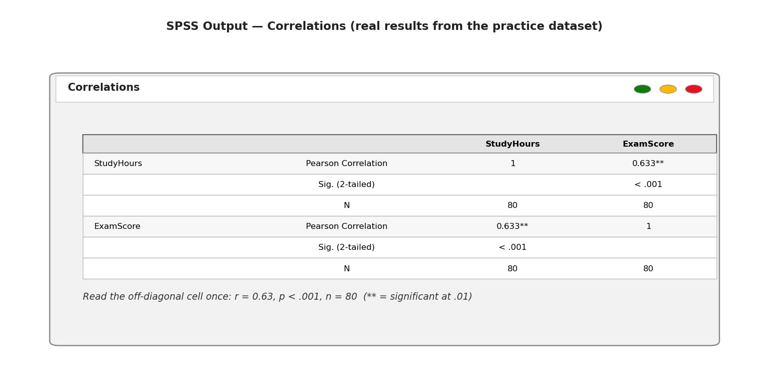
| StudyHours | Pearson Correlation | 1 | .633** |
| Sig. (2-tailed) | < .001 | ||
| N | 80 | 80 | |
| ExamScore | Pearson Correlation | .633** | 1 |
| Sig. (2-tailed) | < .001 | ||
| N | 80 | 80 |
Read the off-diagonal cell — the table is a mirror, so read it once: r = .63, p < .001, n = 80. Positive, significant, and — using Cohen’s benchmarks for r (.10 = small, .30 = medium, .50 = large) — a large effect. Squaring it, r² = .40: about 40% of the variation in exam scores moves together with revision hours. (The ** is just the “flag” you ticked — two stars mean significant at the .01 level.)
This is what the table looks like in your SPSS Output window:
Step 6 — The Scatterplot: Trust, but Verify
A correlation number without a scatterplot is a promise without evidence. The number .63 assumes a straight-line pattern — one wild outlier or a curved cloud can make r lie. So we look: Graphs → Legacy Dialogs → Scatter/Dot… → Simple Scatter, put ExamScore on the Y axis and StudyHours on the X axis, click OK, then double-click the chart and add a fit line (Elements → Fit Line at Total).
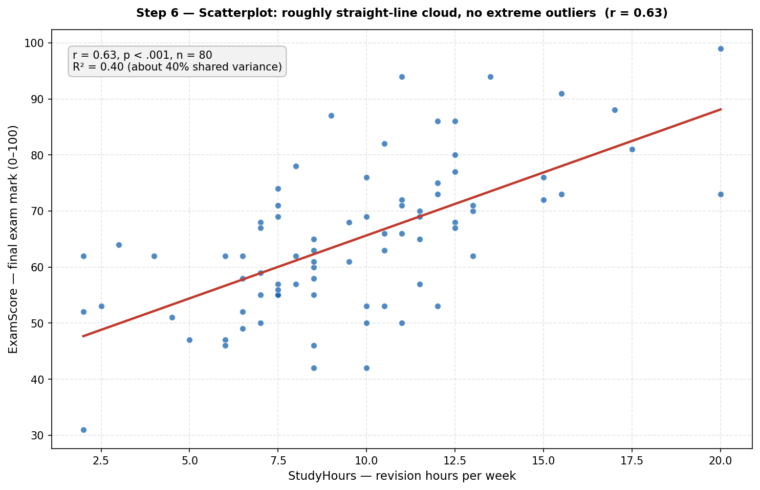
What you should see: a rising cloud of dots, roughly football-shaped, hugging the line — no single dot sitting far away from the rest, no curve. That picture is your licence to trust the .63. If you ever see a U-shape or one extreme dot pulling the line, stop: Pearson is the wrong tool for that picture (consider Spearman, or investigate the outlier).
Writing It Up: The APA-Style Results Paragraph
Here is the complete analysis as a finished results paragraph:
A Pearson correlation was conducted to examine the relationship between weekly revision hours and exam scores. There was a significant, large, positive correlation between revision hours and exam scores, r(78) = .63, p < .001, with students who revised more tending to score higher (revision hours: M = 9.60, SD = 3.75; exam scores: M = 64.75, SD = 13.31). Approximately 40% of the variation in exam scores was shared with revision hours.
Notice the skeleton: what you did, r with degrees of freedom (n − 2 = 78), the p-value, the direction and size in plain words, both means with SDs, then r² translated into an everyday sentence.
So, What Does This Case Study Show?
Two lessons. First, the mechanics: correlation is the simplest analysis in this series — one dialogue box, one table, one number — but the scatterplot is non-negotiable; the number means nothing without the picture. Second, the mindset, unchanged: descriptives first, p-value second, effect size always.
Ready for the next step? Our SPSS help and case studies hub collects every guide — the paired t-test and independent t-test for comparing means, and the one-way ANOVA and two-way ANOVA for when you have more than two groups.
Common Mistakes (and the Calm Fix for Each)
- Reading causation into correlation. r = .63 does not prove revision causes higher scores — motivated students may both revise more and score higher. Write “associated with”, never “caused”, unless your design earns the stronger word.
- Running Pearson on ordinal or curved data. Likert-scale ranks, or a U-shaped scatterplot, need Spearman (same dialogue box, tick Spearman instead). Pearson only describes straight-line relationships between continuous variables.
- Skipping the scatterplot. One extreme outlier can manufacture — or hide — a correlation. Always look at the cloud before you quote the number.
- Reporting r without p and n. “r = .63” alone is incomplete — always give the degrees of freedom, the p-value, and n, so readers can judge the evidence: r(78) = .63, p < .001, n = 80.
- Calling a non-significant r “no relationship”. A non-significant r means no evidence of a linear relationship in this sample — not proof of zero relationship. Report it honestly with its p-value and move on.
You have just run your first correlation — well done.
If choosing the right test is the part you still feel unsure about, take our free workbook: SPSS Dissertation Workbook — Which Test Should You Use? Get the Free Workbook
Prefer something printable? Our Etsy shop has thesis planners and SPSS checklists made for dissertation students.
Also from us: Confident Viva — calm, practical viva preparation for PhD and Masters students.
And if you are working with your own data and would like a second pair of eyes, message us on WhatsApp — tap the icon, tell us where you got stuck, and we will help you find your next step, calmly. No pressure, ever.
Stuck on a step, or did your output look different? Ask in the comments below — we read and reply to every student’s question.
← Previous in this series: How to Run a Paired Samples T-Test in SPSS, Step by Step
A: Use Pearson when both variables are continuous (Scale in SPSS) and their relationship looks roughly straight-line on a scatterplot — like revision hours and exam scores here (r = .63). Use Spearman when a variable is ordinal (rankings, Likert items treated as ranks), the relationship is curved but monotonic, or outliers are pulling Pearson around. Same SPSS dialogue box — just tick a different coefficient.
A: By Cohen’s benchmarks for r: .10 is small, .30 is medium, .50 is large. Our r(78) = .63 is a large effect — and r² = .40 means about 40% of the variation in exam scores moves together with revision hours. But “strong” also depends on your field: in some areas of psychology, .30 is a celebrated finding.
A: No — this is the most important sentence in the whole guide. r = .63, p < .001 tells you revision hours and exam scores move together, not that revision causes higher scores. A third variable (like motivation) could drive both. In your write-up, say “associated with”, never “caused”, unless your research design earns the stronger word.
A: Bigger than you think for small effects: to reliably detect r = .30 you need roughly 85 people; for r = .50, about 30 can do. Our n = 80 was plenty for r = .63 (p < .001). With tiny samples, even a large-looking r may not reach significance — always report n alongside r.
A: Report it honestly, exactly like a significant one: r(df) = .xx, p = .xx, n = xx. A non-significant r means no evidence of a linear relationship in your sample — not proof that no relationship exists. Non-significant findings still belong in your results chapter; hiding them is what biases science.