

Our independent samples t-test case study compared two separate groups of students. But many dissertations measure the same students twice — before and after an intervention, pre-test and post-test. For that, you need the paired samples t-test: the same gentle logic as last time, with one clever twist that makes it more powerful.
In this case study we run a complete paired t-test together: the setup, every click, every output table explained, the effect size, and a finished APA-style results paragraph. One small step at a time.
In this guide
- What a paired samples t-test is — and when to use it
- The case study: does a workshop calm statistics anxiety?
- The hypotheses (one pair, one difference)
- Setting up your data (wide format!)
- Running the test: Steps 1–4
- Reading the output: Steps 5–7
- The APA-style write-up
- Common mistakes (and calm fixes)
- Quick questions, answered
What Is a Paired Samples T-Test (and When Do You Use It)?
A paired samples t-test compares the means of two measurements from the same people — usually before and after something. Use it when:
- The same people were measured twice — pre-test and post-test, before and after.
- You have two timepoints or conditions — not three (that is repeated measures ANOVA, coming soon in this series).
- You measured one continuous outcome both times (an anxiety score, a test mark).
Do not use it for two different groups of people — that is the independent samples t-test we ran last time. The paired test’s clever twist: because each student is their own control, individual differences cancel out, which is why it can detect smaller effects.
The Case Study: Does a Workshop Calm Statistics Anxiety?
The same fictional university, a new question. A lecturer runs a two-hour “Calm Statistics” workshop and wonders whether students’ statistics anxiety genuinely falls afterwards.
40 students completed a statistics anxiety scale (10–50, higher = more anxious) before the workshop and again after it. Same students, same scale, two timepoints.
Research question: is there a difference in mean anxiety scores before and after the workshop?
Why the paired test fits: the same 40 people measured twice on one continuous outcome. An independent t-test here would be wrong — it would treat the before and after scores as if they came from 80 different students.
Practise along with us: download the practice dataset used here — download the free paired t-test practice dataset (CSV) — and follow every step in your own SPSS.
The Hypotheses
One pair of hypotheses, stated as a difference:
- H0 — there is no difference in mean anxiety scores before and after the workshop (mean difference = 0).
- H1 — there is a difference in mean anxiety scores before and after the workshop.
Before You Run Anything: Setting Up the Data
The paired test needs wide format: one row per student, one column per timepoint.
| Variable | Type | Measure | What to set |
|---|---|---|---|
| StudentID | Numeric | Nominal | One row per student (1–40) |
| Before | Numeric | Scale | Anxiety score before the workshop (10–50) |
| After | Numeric | Scale | Anxiety score after the workshop (10–50) |
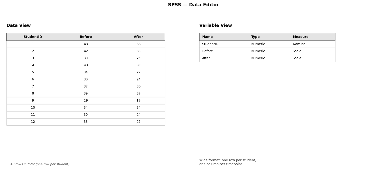
One row per student: an ID, a before score, an after score. If your data is in long format (one row per measurement, 80 rows), restructure it first — the paired test cannot run on long data. Quick sanity check: Descriptives on Before and After to catch impossible values.
Step by Step: Running the Paired T-Test in SPSS
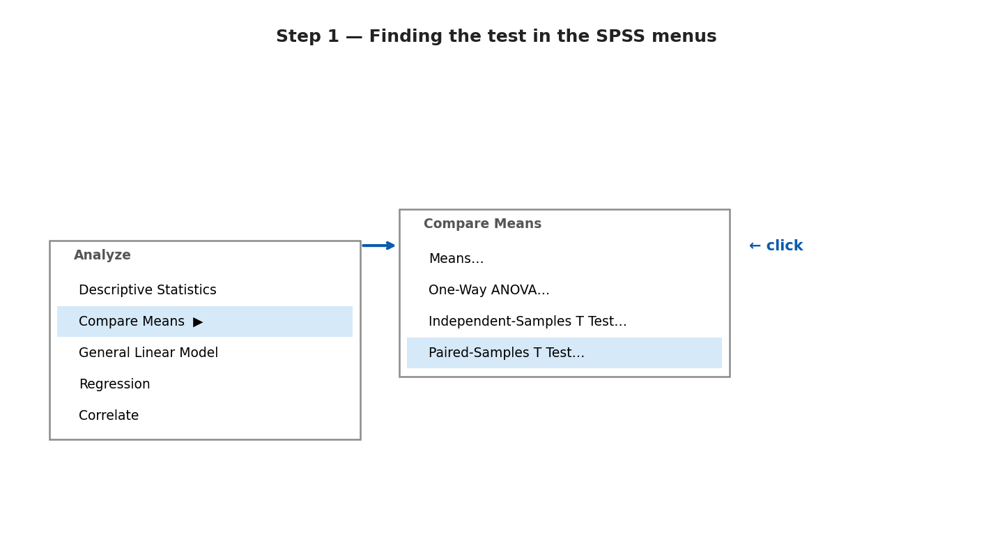
Step 1 — Open the test
Click Analyze → Compare Means → Paired-Samples T Test… A dialogue box opens.
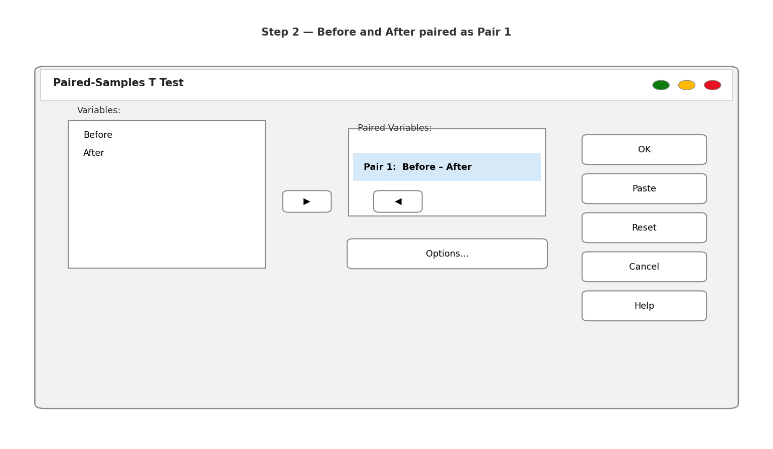
Step 2 — Pair your variables
Move Before and After into the Paired Variables box. SPSS lines them up as Pair 1: Before – After. The order matters for the sign of the difference — keep Before first.
Step 3 — Ask for the effect size
Click Options… and tick Estimate effect sizes. This gives you Cohen’s dz for free — your discussion chapter will thank you.
Step 4 — Run it
Click OK. The Output window opens with three small tables. Smaller than the independent test — the pairing does half the work for you.
Reading the Output, Table by Table
Step 5 — Paired Samples Statistics: Meet Your Two Timepoints
Always start with the means, before any p-value:
Table 1. Paired samples statistics — anxiety score before and after the workshop
| Mean | N | SD | SE | |
|---|---|---|---|---|
| Before | 33.00 | 40 | 5.86 | 0.926 |
| After | 27.30 | 40 | 6.03 | 0.953 |
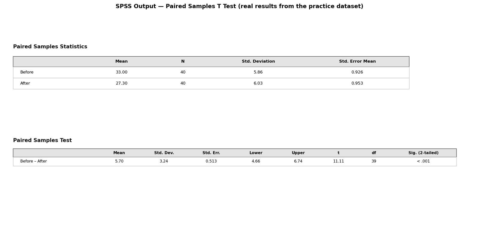
Mean anxiety fell from 33.00 to 27.30 — a drop of about 5.7 points. (SPSS also prints the correlation between the two timepoints: r = 0.85. A decent correlation is good news — it means the pairing is doing its job.) The question, as always: could a drop this size be luck?
Step 6 — The Paired Samples Test: One Difference, One Answer
This table tests a single number: the mean of the difference scores (Before − After for each student).
Table 2. Paired samples test — difference in anxiety scores (Before − After)
| Mean diff. | SD | SE | 95% CI | t | df | Sig. (2-tailed) | |
|---|---|---|---|---|---|---|---|
| Before − After | 5.70 | 3.24 | 0.513 | 4.66 to 6.74 | 11.11 | 39 | < .001 |
Read it in one sweep: the mean difference is 5.70 points, t(39) = 11.11, p < .001. Significant (below .05) — the anxiety drop is not plausibly luck. The 95% confidence interval (4.66 to 6.74) sits entirely above zero, telling the same story in different words.
This is what the tables look like in your SPSS Output window:
Step 7 — Effect Size and the Normality Check
Because you ticked Estimate effect sizes, SPSS prints Cohen’s dz = 1.76 — a large effect (benchmarks: 0.2 = small, 0.5 = medium, 0.8 = large). Significant and practically meaningful: students didn’t just score lower, they scored meaningfully lower.
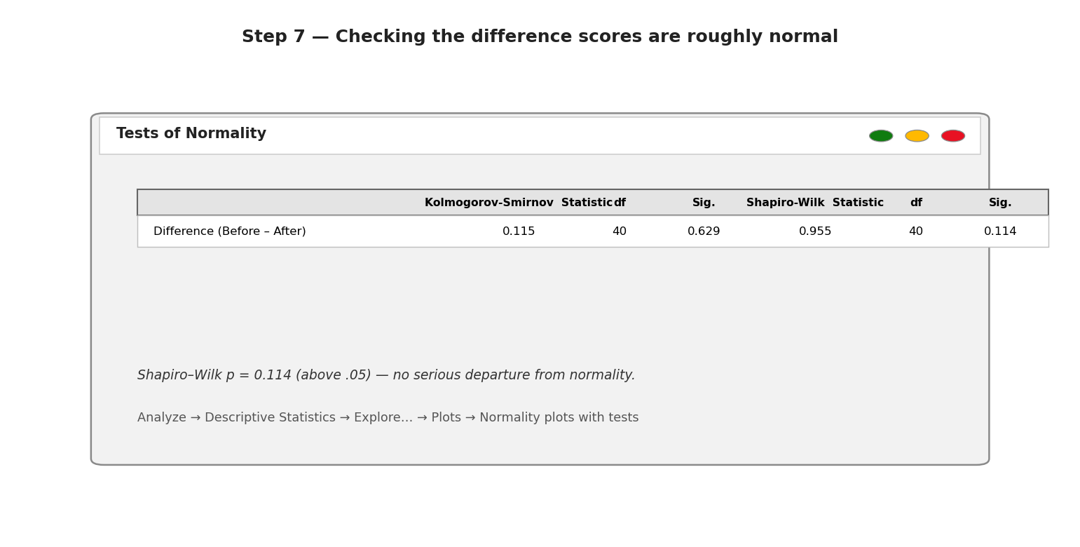
One assumption to glance at: the difference scores should be roughly normal (not the raw before/after scores — a common mix-up). A Shapiro–Wilk test on the differences gives W = 0.955, p = 0.114 — no serious departure from normality, so we proceed calmly.
Writing It Up: The APA-Style Results Paragraph
Here is the complete analysis as a finished results paragraph:
A paired-samples t-test was conducted to compare statistics anxiety scores before and after a calm-statistics workshop. There was a significant decrease in anxiety scores, t(39) = 11.11, p < .001, with lower scores after the workshop (M = 27.30, SD = 6.03) than before it (M = 33.00, SD = 5.86). The mean reduction of 5.70 points, 95% CI [4.66, 6.74], represented a large effect, Cohen’s dz = 1.76.
Notice the skeleton, nearly identical to last time: both means, the test statistic with df, the p-value, the mean difference with its CI, then the effect size in plain words.
So, What Does This Case Study Show?
Two lessons. First, the mechanics: the paired test is the independent test’s cleverer sibling — one dialogue box, one difference score, one clear answer, and more power because each student controls for themselves. Second, the mindset, unchanged: means first, p-value second, effect size always.
Ready for the next step? Our SPSS help and case studies hub collects every guide — including the one-way ANOVA and two-way ANOVA case studies for when you have more than two groups, and the independent samples t-test for when your groups are different people.
Common Mistakes (and the Calm Fix for Each)
- Using an independent t-test on paired data. Same students twice needs the paired test — the independent version ignores the pairing and throws away power. If each row is a person measured twice, it is paired.
- Entering data in long format. One row per measurement (80 rows) will not run. Restructure to wide format first: one row per student, one column per timepoint.
- Mixing up the direction of the difference. SPSS subtracts the second variable from the first (Before − After). A positive t here means before was higher — anxiety fell. Always check which way round your pair is before interpreting.
- Checking normality of the wrong thing. The assumption is about the difference scores, not the before and after scores separately. One Shapiro–Wilk on the differences is all you need.
- Reporting p without the means and dz. “p < .001” alone says nothing about how much anxiety fell — always give both timepoint means, the mean difference, and the effect size.
You have just run your first paired t-test — well done.
If choosing the right test is the part you still feel unsure about, take our free workbook: SPSS Dissertation Workbook — Which Test Should You Use? Get the Free Workbook
Prefer something printable? Our Etsy shop has thesis planners and SPSS checklists made for dissertation students.
Also from us: Confident Viva — calm, practical viva preparation for PhD and Masters students.
And if you are working with your own data and would like a second pair of eyes, message us on WhatsApp — tap the icon, tell us where you got stuck, and we will help you find your next step, calmly. No pressure, ever.
Stuck on a step, or did your output look different? Ask in the comments below — we read and reply to every student’s question.
← Previous in this series: How to Run an Independent Samples T-Test in SPSS, Step by Step
Paired compares the same people measured twice (before/after — like here); independent compares two different groups of people. Different designs, different SPSS dialogue boxes — our independent samples t-test case study covers the other one.
With 40 pairs, the t-test is quite forgiving. With small or badly skewed differences, use the non-parametric alternative: the Wilcoxon signed-rank test (Analyze → Nonparametric Tests → Related Samples).
No — the paired t-test only handles two measurements. Three or more timepoints need a repeated measures ANOVA (one-way within-subjects) — coming soon in this series.
The paired test uses complete pairs only, so those students drop out of this analysis — report your final n honestly (here, 40). If many are missing, pause and think about why before deleting anyone.
Both timepoint means with SDs, the mean difference with its 95% confidence interval, t with degrees of freedom, the exact p-value, and Cohen’s dz. That is the full story in one paragraph.